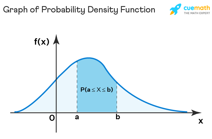
Probability density function is a function that provides the likelihood that the value of a random variable will fall between a certain range of values. We use the probability density function in the case of continuous random variables. For discrete random variables, we use the probability mass function which is analogous to the probability density function.
The graph of a probability density function is in the form of a bell curve. The area that lies between any two specified values gives the probability of the outcome of the designated observation. We solve the integral of this function to determine the probabilities associated with a continuous random variable. In this article, we will do a detailed analysis of the probability density function and take a look at the various aspects related to it.
| 1. | What is Probability Density Function? |
| 2. | Probability Density Function Formula |
| 3. | Mean of Probability Density Function |
| 4. | Median of Probability Density Function |
| 5. | Variance of Probability Density Function |
| 6. | Properties of Probability Density Function |
| 7. | FAQs on Probability Density Function |
Probability density function and cumulative distribution function are used to define the distribution of continuous random variables. If we differentiate the cumulative distribution function of a continuous random variable it results in the probability density function. Conversely, on integrating the probability density function we get the cumulative distribution function.
Probability density function defines the density of the probability that a continuous random variable will lie within a particular range of values. To determine this probability, we integrate the probability density function between two specified points.
The probability density function of a continuous random variable is analogous to the probability mass function of a discrete random variable. Discrete random variables can be evaluated at a particular point while continuous random variables have to be evaluated between a certain interval. This is because the probability that a continuous random variable will take an exact value is 0. Given below are the various probability density function formulas.
Suppose we have a continuous random variable, X. Let F(x) be the cumulative distribution function of X. Then the formula for the probability density function, f(x), is given as follows:
If we want to find the probability that X lies between lower limit 'a' and upper limit 'b' then using the probability density function this can be given as:
Here, F(b) and F(a) represent the cumulative distribution function at b and a respectively.
Normal distribution is the most widely used type of continuous probability distribution. The notation for normal distribution is given as \(X \sim N(\mu ,\sigma ^)\). The probability density function of a normal distribution is given below.
Here, \(\mu\) is the mean and \(\sigma\) is the standard deviation while \(\sigma\) 2 is the variance.
If X is a continuous random variable then the probability distribution of this variable is given by the probability density function. The graph given below depicts the probability that X will lie between two points a and b.

In the case of a probability density function, the mean is the expected value or the average value of the random variable. If f(x) is the probability density function of the random variable X, then mean is given by the following formula:
The median is the value that splits the probability density function curve into two equal halves. Suppose x = m is the value of the median. The area under the curve from \(-\infty\) to m will be equal to the area under the curve from m to \(\infty\). This implies that the value of the median is 1 / 2. Thus, the median of the probability density function is given as follows:

The expected value of the squared deviation from the mean is the variance of a random variable. Expressing this definition mathematically we get,
To represent this variance with the help of the probability density function, the formula is given as:
The properties of the probability density function help to solve questions faster. If f(x) is the probability distribution of a continuous random variable, X, then some of the useful properties are listed below:
Related Articles:
Important Notes on Probability Density Function
Example 1: If the probability density function is given as:
f(x) = \(\left\ x(x-1) &0\leq x < 3 \\ x& x\geq3 \end\right.\)
Find P(1 < X < 2).
Solution: Integrating the function,
\(\int_^x(x-1)dx\) = \(\int_^(x^-x)dx\)
= \([\frac> - \frac
= 5 / 6
Answer: P(1< X < 2) = 5 / 6
Example 2: If X is a continuous random variable with the probability density function given as:
f(x) = \(\left\ \frac> & x\geq 0\\ 0 & \text \end\right.\)
Find the value of b.
Solution: We know from properties of probability density function that \(\int_<-\infty >^<\infty>f(x)dx\) = 1
\(\int_^<\infty >\frac>dx\) = 1
On integrating,
\(\frac\left [ -e^ \right ]_^<\infty >\) = 1
b / 2 = 1
b = 2
Answer: b = 2
Example 3: Find the expected value of X if the probability density function is defined as:
f(x) = \(\left\ \fracx^ & 0\leq x\leq 2\\ 0& \text \end\right.\)
Solution: We know that, E[X] = \(\int_<-\infty >^<\infty>xf(x)dx\)
= \(\int_<-\infty >^x(0)dx + \int_^x (\frac<3x^>)dx + \int_^<\infty >x(0)dx\)
= \(\frac[\frac>]_^\)
= (3/8) [16]
= 6
Answer: Mean = 6

Math will no longer be a tough subject, especially when you understand the concepts through visualizations.